healpy tutorial¶

See the Jupyter Notebook version of this tutorial at https://github.com/healpy/healpy/blob/master/doc/tutorial.ipynb

Choose the inline backend of maptlotlib to display the plots inside the Jupyter Notebook

[1]:

import matplotlib.pyplot as plt

%matplotlib inline

[2]:

import numpy as np
import healpy as hp

NSIDE and ordering¶

Maps are simply numpy arrays, where each array element refers to a location in the sky as defined by the Healpix pixelization schemes (see the healpix website).

Note: Running the code below in a regular Python session will not display the maps; it’s recommended to use an IPython shell or a Jupyter notebook.

The resolution of the map is defined by the NSIDE parameter, which is generally a power of 2.

[3]:

NSIDE = 32
print(
    "Approximate resolution at NSIDE {} is {:.2} deg".format(
        NSIDE, hp.nside2resol(NSIDE, arcmin=True) / 60
    )
)

Approximate resolution at NSIDE 32 is 1.8 deg

The function healpy.pixelfunc.nside2npix gives the number of pixels NPIX of the map:

[4]:

NPIX = hp.nside2npix(NSIDE)
print(NPIX)

The same pixels in the map can be ordered in 2 ways, either RING, where they are numbered in the array in horizontal rings starting from the North pole:

[5]:

m = np.arange(NPIX)
hp.mollview(m, title="Mollview image RING")
hp.graticule()

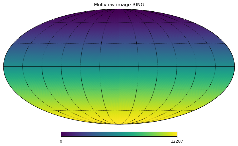
The standard coordinates are the colatitude \(\theta\), \(0\) at the North Pole, \(\pi/2\) at the equator and \(\pi\) at the South Pole and the longitude \(\phi\) between \(0\) and \(2\pi\) eastward, in a Mollview projection, \(\phi=0\) is at the center and increases eastward toward the left of the map.

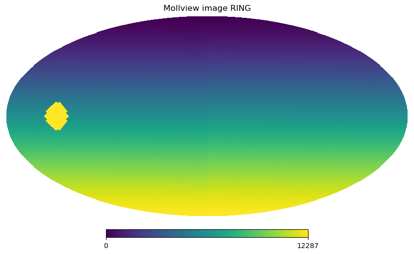
We can also use vectors to represent coordinates, for example vec is the normalized vector that points to \(\theta=\pi/2, \phi=3/4\pi\):

[6]:

vec = hp.ang2vec(np.pi / 2, np.pi * 3 / 4)
print(vec)

[-7.07106781e-01  7.07106781e-01  6.12323400e-17]

We can find the indices of all the pixels within \(10\) degrees of that point and then change the value of the map at those indices:

[7]:

ipix_disc = hp.query_disc(nside=32, vec=vec, radius=np.radians(10))

[8]:

m = np.arange(NPIX)
m[ipix_disc] = m.max()
hp.mollview(m, title="Mollview image RING")

We can retrieve colatitude and longitude of each pixel using pix2ang, in this case we notice that the first 4 pixels cover the North Pole with pixel centers just ~\(1.5\) degrees South of the Pole all at the same latitude. The fifth pixel is already part of another ring of pixels.

[9]:

theta, phi = np.degrees(hp.pix2ang(nside=32, ipix=[0, 1, 2, 3, 4]))

[10]:

theta

[10]:

array([1.46197116, 1.46197116, 1.46197116, 1.46197116, 2.92418036])

[11]:

phi

[11]:

array([ 45. , 135. , 225. , 315. ,  22.5])

The RING ordering is necessary for the Spherical Harmonics transforms, the other option is NESTED ordering which is very efficient for map domain operations because scaling up and down maps is achieved just multiplying and rounding pixel indices. See below how pixel are ordered in the NESTED scheme, notice the structure of the 12 HEALPix base pixels (NSIDE 1):

[12]:

m = np.arange(NPIX)
hp.mollview(m, nest=True, title="Mollview image NESTED")

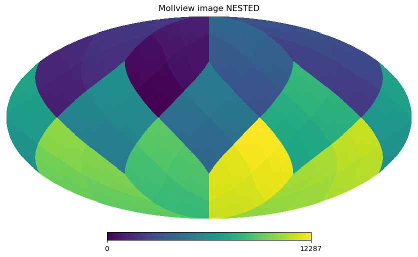
All healpy routines assume RING ordering, in fact as soon as you read a map with read_map, even if it was stored as NESTED, it is transformed to RING. However, you can work in NESTED ordering passing the nest=True argument to most healpy routines.

Reading and writing maps to file¶

For the following section, it is required to download larger maps by executing from the terminal the bash script healpy_get_wmap_maps.sh which should be available in your path.

This will download the higher resolution WMAP data into the current directory.

[13]:

!wget -c http://lambda.gsfc.nasa.gov/data/map/dr4/skymaps/7yr/raw/wmap_band_iqumap_r9_7yr_W_v4.fits;wget -c http://lambda.gsfc.nasa.gov/data/map/dr4/ancillary/masks/wmap_temperature_analysis_mask_r9_7yr_v4.fits

--2024-04-22 23:33:43--  http://lambda.gsfc.nasa.gov/data/map/dr4/skymaps/7yr/raw/wmap_band_iqumap_r9_7yr_W_v4.fits
Resolving lambda.gsfc.nasa.gov (lambda.gsfc.nasa.gov)...

129.164.179.68, 2001:4d0:2310:150::68
Connecting to lambda.gsfc.nasa.gov (lambda.gsfc.nasa.gov)|129.164.179.68|:80... connected.
HTTP request sent, awaiting response...

301 Moved Permanently
Location: https://lambda.gsfc.nasa.gov/data/map/dr4/skymaps/7yr/raw/wmap_band_iqumap_r9_7yr_W_v4.fits [following]
--2024-04-22 23:33:44--  https://lambda.gsfc.nasa.gov/data/map/dr4/skymaps/7yr/raw/wmap_band_iqumap_r9_7yr_W_v4.fits
Connecting to lambda.gsfc.nasa.gov (lambda.gsfc.nasa.gov)|129.164.179.68|:443... connected.

HTTP request sent, awaiting response... 200 OK
Length: 100676160 (96M)
Saving to: ‘wmap_band_iqumap_r9_7yr_W_v4.fits’


  wmap_band   0%[                    ]       0  --.-KB/s


 wmap_band_   0%[                    ] 288.91K  1.38MB/s


wmap_band_i   0%[                    ] 781.09K  1.88MB/s


wmap_band_iq   1%[                    ]   1.66M  2.73MB/s


wmap_band_iqu   3%[                    ]   3.26M  4.05MB/s


wmap_band_iqum   5%[>                   ]   4.94M  4.91MB/s

wmap_band_iquma 7%[> ] 6.90M 5.72MB/s: </pre>

wmap_band_iquma 7%[> ] 6.90M 5.72MB/s: end{sphinxVerbatim}

wmap_band_iquma 7%[> ] 6.90M 5.72MB/s

more-to-come:

wmap_band_iqumap 9%[> ] 8.99M 6.40MB/s: </pre>
wmap_band_iqumap 9%[> ] 8.99M 6.40MB/s: end{sphinxVerbatim}

wmap_band_iqumap 9%[> ] 8.99M 6.40MB/s

more-to-come:

wmap_band_iqumap_ 11%[=> ] 10.95M 6.81MB/s: </pre>
wmap_band_iqumap_ 11%[=> ] 10.95M 6.81MB/s: end{sphinxVerbatim}

wmap_band_iqumap_ 11%[=> ] 10.95M 6.81MB/s

more-to-come:

wmap_band_iqumap_r 13%[=> ] 13.03M 7.21MB/s: </pre>
wmap_band_iqumap_r 13%[=> ] 13.03M 7.21MB/s: end{sphinxVerbatim}

wmap_band_iqumap_r 13%[=> ] 13.03M 7.21MB/s

wmap_band_iqumap_r9 15%[==> ] 15.12M 7.53MB/s: </pre>
wmap_band_iqumap_r9 15%[==> ] 15.12M 7.53MB/s: end{sphinxVerbatim}

wmap_band_iqumap_r9 15%[==> ] 15.12M 7.53MB/s

map_band_iqumap_r9_ 17%[==> ] 17.09M 7.74MB/s: </pre>
map_band_iqumap_r9_ 17%[==> ] 17.09M 7.74MB/s: end{sphinxVerbatim}

map_band_iqumap_r9_ 17%[==> ] 17.09M 7.74MB/s

ap_band_iqumap_r9_7 19%[==> ] 19.19M 7.96MB/s: </pre>
ap_band_iqumap_r9_7 19%[==> ] 19.19M 7.96MB/s: end{sphinxVerbatim}

ap_band_iqumap_r9_7 19%[==> ] 19.19M 7.96MB/s

p_band_iqumap_r9_7y 22%[===> ] 21.25M 8.13MB/s: </pre>
p_band_iqumap_r9_7y 22%[===> ] 21.25M 8.13MB/s: end{sphinxVerbatim}

p_band_iqumap_r9_7y 22%[===> ] 21.25M 8.13MB/s

_band_iqumap_r9_7yr 24%[===> ] 23.37M 8.30MB/s: </pre>
_band_iqumap_r9_7yr 24%[===> ] 23.37M 8.30MB/s: end{sphinxVerbatim}

_band_iqumap_r9_7yr 24%[===> ] 23.37M 8.30MB/s

band_iqumap_r9_7yr_ 26%[====> ] 25.47M 8.45MB/s eta 8s: </pre>
band_iqumap_r9_7yr_ 26%[====> ] 25.47M 8.45MB/s eta 8s: end{sphinxVerbatim}

band_iqumap_r9_7yr_ 26%[====> ] 25.47M 8.45MB/s eta 8s

and_iqumap_r9_7yr_W 28%[====> ] 27.59M 8.94MB/s eta 8s: </pre>
and_iqumap_r9_7yr_W 28%[====> ] 27.59M 8.94MB/s eta 8s: end{sphinxVerbatim}

and_iqumap_r9_7yr_W 28%[====> ] 27.59M 8.94MB/s eta 8s

nd_iqumap_r9_7yr_W_ 30%[=====> ] 29.59M 9.35MB/s eta 8s: </pre>
nd_iqumap_r9_7yr_W_ 30%[=====> ] 29.59M 9.35MB/s eta 8s: end{sphinxVerbatim}

nd_iqumap_r9_7yr_W_ 30%[=====> ] 29.59M 9.35MB/s eta 8s

d_iqumap_r9_7yr_W_v 33%[=====> ] 31.70M 9.72MB/s eta 8s: </pre>
d_iqumap_r9_7yr_W_v 33%[=====> ] 31.70M 9.72MB/s eta 8s: end{sphinxVerbatim}

d_iqumap_r9_7yr_W_v 33%[=====> ] 31.70M 9.72MB/s eta 8s

_iqumap_r9_7yr_W_v4 35%[======> ] 33.74M 10.1MB/s eta 8s: </pre>
_iqumap_r9_7yr_W_v4 35%[======> ] 33.74M 10.1MB/s eta 8s: end{sphinxVerbatim}

_iqumap_r9_7yr_W_v4 35%[======> ] 33.74M 10.1MB/s eta 8s

iqumap_r9_7yr_W_v4. 37%[======> ] 35.86M 10.2MB/s eta 7s: </pre>
iqumap_r9_7yr_W_v4. 37%[======> ] 35.86M 10.2MB/s eta 7s: end{sphinxVerbatim}

iqumap_r9_7yr_W_v4. 37%[======> ] 35.86M 10.2MB/s eta 7s

qumap_r9_7yr_W_v4.f 39%[======> ] 37.96M 10.3MB/s eta 7s: </pre>
qumap_r9_7yr_W_v4.f 39%[======> ] 37.96M 10.3MB/s eta 7s: end{sphinxVerbatim}

qumap_r9_7yr_W_v4.f 39%[======> ] 37.96M 10.3MB/s eta 7s

umap_r9_7yr_W_v4.fi 41%[=======> ] 40.08M 10.3MB/s eta 7s: </pre>
umap_r9_7yr_W_v4.fi 41%[=======> ] 40.08M 10.3MB/s eta 7s: end{sphinxVerbatim}

umap_r9_7yr_W_v4.fi 41%[=======> ] 40.08M 10.3MB/s eta 7s

map_r9_7yr_W_v4.fit 43%[=======> ] 42.09M 10.3MB/s eta 7s: </pre>
map_r9_7yr_W_v4.fit 43%[=======> ] 42.09M 10.3MB/s eta 7s: end{sphinxVerbatim}

map_r9_7yr_W_v4.fit 43%[=======> ] 42.09M 10.3MB/s eta 7s

ap_r9_7yr_W_v4.fits 46%[========> ] 44.19M 10.3MB/s eta 7s: </pre>
ap_r9_7yr_W_v4.fits 46%[========> ] 44.19M 10.3MB/s eta 7s: end{sphinxVerbatim}

ap_r9_7yr_W_v4.fits 46%[========> ] 44.19M 10.3MB/s eta 7s

p_r9_7yr_W_v4.fits 48%[========> ] 46.29M 10.3MB/s eta 5s: </pre>
p_r9_7yr_W_v4.fits 48%[========> ] 46.29M 10.3MB/s eta 5s: end{sphinxVerbatim}

p_r9_7yr_W_v4.fits 48%[========> ] 46.29M 10.3MB/s eta 5s

_r9_7yr_W_v4.fits 50%[=========> ] 48.39M 10.4MB/s eta 5s: </pre>
_r9_7yr_W_v4.fits 50%[=========> ] 48.39M 10.4MB/s eta 5s: end{sphinxVerbatim}

_r9_7yr_W_v4.fits 50%[=========> ] 48.39M 10.4MB/s eta 5s

r9_7yr_W_v4.fits 52%[=========> ] 50.39M 10.4MB/s eta 5s: </pre>
r9_7yr_W_v4.fits 52%[=========> ] 50.39M 10.4MB/s eta 5s: end{sphinxVerbatim}

r9_7yr_W_v4.fits 52%[=========> ] 50.39M 10.4MB/s eta 5s

9_7yr_W_v4.fits 54%[=========> ] 52.50M 10.4MB/s eta 5s: </pre>
9_7yr_W_v4.fits 54%[=========> ] 52.50M 10.4MB/s eta 5s: end{sphinxVerbatim}

9_7yr_W_v4.fits 54%[=========> ] 52.50M 10.4MB/s eta 5s

_7yr_W_v4.fits 56%[==========> ] 54.61M 10.4MB/s eta 5s: </pre>
_7yr_W_v4.fits 56%[==========> ] 54.61M 10.4MB/s eta 5s: end{sphinxVerbatim}

_7yr_W_v4.fits 56%[==========> ] 54.61M 10.4MB/s eta 5s

7yr_W_v4.fits 59%[==========> ] 56.71M 10.4MB/s eta 4s: </pre>
7yr_W_v4.fits 59%[==========> ] 56.71M 10.4MB/s eta 4s: end{sphinxVerbatim}

7yr_W_v4.fits 59%[==========> ] 56.71M 10.4MB/s eta 4s

yr_W_v4.fits 61%[===========> ] 58.71M 10.3MB/s eta 4s: </pre>
yr_W_v4.fits 61%[===========> ] 58.71M 10.3MB/s eta 4s: end{sphinxVerbatim}

yr_W_v4.fits 61%[===========> ] 58.71M 10.3MB/s eta 4s

r_W_v4.fits 63%[===========> ] 60.83M 10.4MB/s eta 4s: </pre>
r_W_v4.fits 63%[===========> ] 60.83M 10.4MB/s eta 4s: end{sphinxVerbatim}

r_W_v4.fits 63%[===========> ] 60.83M 10.4MB/s eta 4s

_W_v4.fits 65%[============> ] 62.93M 10.4MB/s eta 4s: </pre>
_W_v4.fits 65%[============> ] 62.93M 10.4MB/s eta 4s: end{sphinxVerbatim}

_W_v4.fits 65%[============> ] 62.93M 10.4MB/s eta 4s

W_v4.fits 67%[============> ] 64.93M 10.4MB/s eta 4s: </pre>
W_v4.fits 67%[============> ] 64.93M 10.4MB/s eta 4s: end{sphinxVerbatim}

W_v4.fits 67%[============> ] 64.93M 10.4MB/s eta 4s

_v4.fits 69%[============> ] 67.03M 10.4MB/s eta 3s: </pre>
_v4.fits 69%[============> ] 67.03M 10.4MB/s eta 3s: end{sphinxVerbatim}

_v4.fits 69%[============> ] 67.03M 10.4MB/s eta 3s

v4.fits 72%[=============> ] 69.14M 10.4MB/s eta 3s: </pre>
v4.fits 72%[=============> ] 69.14M 10.4MB/s eta 3s: end{sphinxVerbatim}

v4.fits 72%[=============> ] 69.14M 10.4MB/s eta 3s

4.fits 74%[=============> ] 71.24M 10.4MB/s eta 3s: </pre>
4.fits 74%[=============> ] 71.24M 10.4MB/s eta 3s: end{sphinxVerbatim}

4.fits 74%[=============> ] 71.24M 10.4MB/s eta 3s

.fits 76%[==============> ] 73.34M 10.4MB/s eta 3s: </pre>
.fits 76%[==============> ] 73.34M 10.4MB/s eta 3s: end{sphinxVerbatim}

.fits 76%[==============> ] 73.34M 10.4MB/s eta 3s

fits 78%[==============> ] 75.45M 10.4MB/s eta 3s: </pre>
fits 78%[==============> ] 75.45M 10.4MB/s eta 3s: end{sphinxVerbatim}

fits 78%[==============> ] 75.45M 10.4MB/s eta 3s

its 80%[===============> ] 77.55M 10.4MB/s eta 2s: </pre>
its 80%[===============> ] 77.55M 10.4MB/s eta 2s: end{sphinxVerbatim}

its 80%[===============> ] 77.55M 10.4MB/s eta 2s

ts 82%[===============> ] 79.67M 10.4MB/s eta 2s: </pre>
ts 82%[===============> ] 79.67M 10.4MB/s eta 2s: end{sphinxVerbatim}

ts 82%[===============> ] 79.67M 10.4MB/s eta 2s

s 85%[================> ] 81.78M 10.4MB/s eta 2s: </pre>
s 85%[================> ] 81.78M 10.4MB/s eta 2s: end{sphinxVerbatim}

s 85%[================> ] 81.78M 10.4MB/s eta 2s


             87%[================>   ]  83.59M  10.3MB/s    eta 2s


          w  89%[================>   ]  85.70M  10.3MB/s    eta 2s


         wm  91%[=================>  ]  87.81M  10.3MB/s    eta 1s


        wma  93%[=================>  ]  89.92M  10.3MB/s    eta 1s


       wmap  95%[==================> ]  92.03M  10.3MB/s    eta 1s


      wmap_  98%[==================> ]  94.13M  10.3MB/s    eta 1s

wmap_band_iqumap_r9 100%[===================>] 96.01M 10.4MB/s in 9.8s

2024-04-22 23:33:54 (9.78 MB/s) - ‘wmap_band_iqumap_r9_7yr_W_v4.fits’ saved [100676160/100676160]

URL transformed to HTTPS due to an HSTS policy –2024-04-22 23:33:54– https://lambda.gsfc.nasa.gov/data/map/dr4/ancillary/masks/wmap_temperature_analysis_mask_r9_7yr_v4.fits Resolving lambda.gsfc.nasa.gov (lambda.gsfc.nasa.gov)… 129.164.179.68, 2001:4d0:2310:150::68 Connecting to lambda.gsfc.nasa.gov (lambda.gsfc.nasa.gov)|129.164.179.68|:443… connected. </pre>

wmap_band_iqumap_r9 100%[===================>] 96.01M 10.4MB/s in 9.8s

2024-04-22 23:33:54 (9.78 MB/s) - ‘wmap_band_iqumap_r9_7yr_W_v4.fits’ saved [100676160/100676160]

URL transformed to HTTPS due to an HSTS policy –2024-04-22 23:33:54– https://lambda.gsfc.nasa.gov/data/map/dr4/ancillary/masks/wmap_temperature_analysis_mask_r9_7yr_v4.fits Resolving lambda.gsfc.nasa.gov (lambda.gsfc.nasa.gov){ldots} 129.164.179.68, 2001:4d0:2310:150::68 Connecting to lambda.gsfc.nasa.gov (lambda.gsfc.nasa.gov)|129.164.179.68|:443{ldots} connected. end{sphinxVerbatim}

wmap_band_iqumap_r9 100%[===================>] 96.01M 10.4MB/s in 9.8s

2024-04-22 23:33:54 (9.78 MB/s) - ‘wmap_band_iqumap_r9_7yr_W_v4.fits’ saved [100676160/100676160]

URL transformed to HTTPS due to an HSTS policy –2024-04-22 23:33:54– https://lambda.gsfc.nasa.gov/data/map/dr4/ancillary/masks/wmap_temperature_analysis_mask_r9_7yr_v4.fits Resolving lambda.gsfc.nasa.gov (lambda.gsfc.nasa.gov)… 129.164.179.68, 2001:4d0:2310:150::68 Connecting to lambda.gsfc.nasa.gov (lambda.gsfc.nasa.gov)|129.164.179.68|:443… connected.

HTTP request sent, awaiting response... 200 OK
Length: 25174080 (24M)
Saving to: ‘wmap_temperature_analysis_mask_r9_7yr_v4.fits’


  wmap_temp   0%[                    ]       0  --.-KB/s


 wmap_tempe   5%[>                   ]   1.30M  6.52MB/s


wmap_temper  12%[=>                  ]   2.96M  7.39MB/s


wmap_tempera  21%[===>                ]   5.07M  8.43MB/s


wmap_temperat  29%[====>               ]   7.03M  8.77MB/s


wmap_temperatu  38%[======>             ]   9.14M  9.13MB/s

wmap_temperatur 46%[========> ] 11.25M 9.36MB/s: </pre>

wmap_temperatur 46%[========> ] 11.25M 9.36MB/s: end{sphinxVerbatim}

wmap_temperatur 46%[========> ] 11.25M 9.36MB/s

more-to-come:

wmap_temperature 55%[==========> ] 13.33M 9.44MB/s: </pre>
wmap_temperature 55%[==========> ] 13.33M 9.44MB/s: end{sphinxVerbatim}

wmap_temperature 55%[==========> ] 13.33M 9.44MB/s

more-to-come:

wmap_temperature_ 64%[===========> ] 15.45M 9.58MB/s: </pre>
wmap_temperature_ 64%[===========> ] 15.45M 9.58MB/s: end{sphinxVerbatim}

wmap_temperature_ 64%[===========> ] 15.45M 9.58MB/s

more-to-come:

wmap_temperature_a 72%[=============> ] 17.40M 9.60MB/s: </pre>
wmap_temperature_a 72%[=============> ] 17.40M 9.60MB/s: end{sphinxVerbatim}

wmap_temperature_a 72%[=============> ] 17.40M 9.60MB/s

wmap_temperature_an 81%[===============> ] 19.52M 9.67MB/s: </pre>
wmap_temperature_an 81%[===============> ] 19.52M 9.67MB/s: end{sphinxVerbatim}

wmap_temperature_an 81%[===============> ] 19.52M 9.67MB/s

map_temperature_ana 90%[=================> ] 21.63M 9.75MB/s: </pre>
map_temperature_ana 90%[=================> ] 21.63M 9.75MB/s: end{sphinxVerbatim}

map_temperature_ana 90%[=================> ] 21.63M 9.75MB/s

ap_temperature_anal 98%[==================> ] 23.73M 9.81MB/s wmap_temperature_an 100%[===================>] 24.01M 9.82MB/s in 2.4s

2024-04-22 23:33:56 (9.82 MB/s) - ‘wmap_temperature_analysis_mask_r9_7yr_v4.fits’ saved [25174080/25174080]

</pre>

ap_temperature_anal 98%[==================> ] 23.73M 9.81MB/s wmap_temperature_an 100%[===================>] 24.01M 9.82MB/s in 2.4s

2024-04-22 23:33:56 (9.82 MB/s) - ‘wmap_temperature_analysis_mask_r9_7yr_v4.fits’ saved [25174080/25174080]

end{sphinxVerbatim}

ap_temperature_anal 98%[==================> ] 23.73M 9.81MB/s wmap_temperature_an 100%[===================>] 24.01M 9.82MB/s in 2.4s

2024-04-22 23:33:56 (9.82 MB/s) - ‘wmap_temperature_analysis_mask_r9_7yr_v4.fits’ saved [25174080/25174080]

[14]:

wmap_map_I = hp.read_map("wmap_band_iqumap_r9_7yr_W_v4.fits")

By default, input maps are converted to RING ordering, if they are in NESTED ordering. You can otherwise specify nest=True to retrieve a map is NESTED ordering, or nest=None to keep the ordering unchanged.

By default, read_map loads the first column, for reading other columns you can specify the field keyword.

write_map writes a map to disk in FITS format, if the input map is a list of 3 maps, they are written to a single file as I,Q,U polarization components:

[15]:

hp.write_map("my_map.fits", wmap_map_I, overwrite=True)

setting the output map dtype to [dtype('>f4')]

Visualization¶

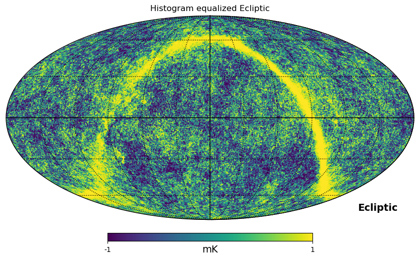
As shown above, mollweide projection with mollview is the most common visualization tool for HEALPIX maps. It also supports coordinate transformation, coord does Galactic to ecliptic coordinate transformation, norm='hist' sets a histogram equalized color scale and xsize increases the size of the image. graticule adds meridians and parallels.

[16]:

hp.mollview(
    wmap_map_I,
    coord=["G", "E"],
    title="Histogram equalized Ecliptic",
    unit="mK",
    norm="hist",
    min=-1,
    max=1,
)
hp.graticule()

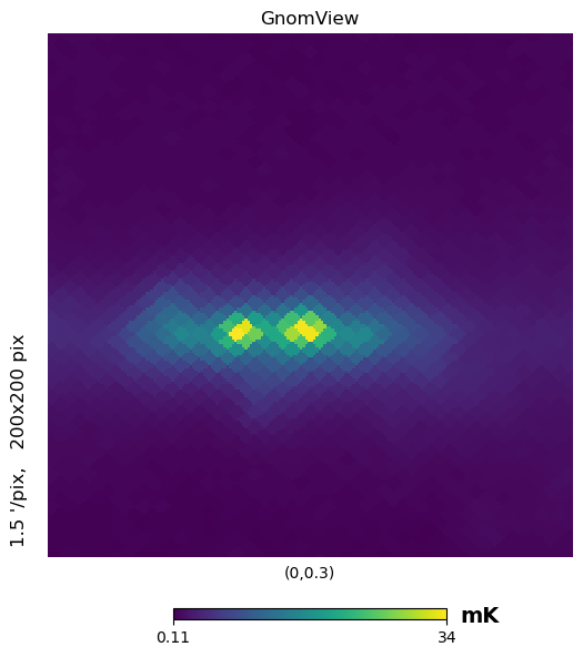
gnomview instead provides gnomonic projection around a position specified by rot, for example you can plot a projection of the galactic center, xsize and ysize change the dimension of the sky patch.

[17]:

hp.gnomview(wmap_map_I, rot=[0, 0.3], title="GnomView", unit="mK", format="%.2g")

mollzoom is a powerful tool for interactive inspection of a map, it provides a mollweide projection where you can click to set the center of the adjacent gnomview panel. ## Masked map, partial maps

By convention, HEALPIX uses \(-1.6375 * 10^{30}\) to mark invalid or unseen pixels. This is stored in healpy as the constant UNSEEN.

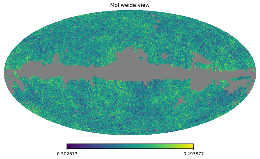
All healpy functions automatically deal with maps with UNSEEN pixels, for example mollview marks in grey those sections of a map.

There is an alternative way of dealing with UNSEEN pixel based on the numpyMaskedArray class, hp.ma loads a map as a masked array, by convention the mask is 0 where the data are masked, while numpy defines data masked when the mask is True, so it is necessary to flip the mask.

[18]:

mask = hp.read_map("wmap_temperature_analysis_mask_r9_7yr_v4.fits").astype(np.bool_)
wmap_map_I_masked = hp.ma(wmap_map_I)
wmap_map_I_masked.mask = np.logical_not(mask)

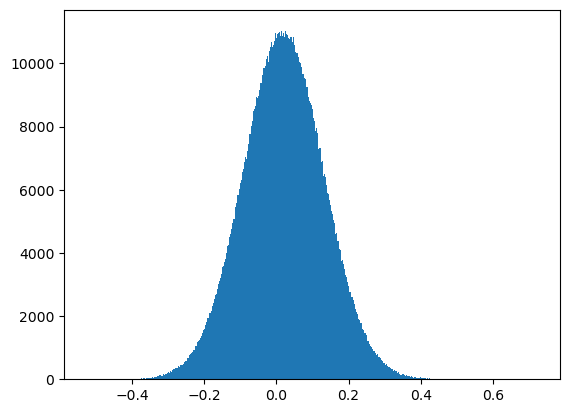
Filling a masked array fills in the UNSEEN value and return a standard array that can be used by mollview. compressed() instead removes all the masked pixels and returns a standard array that can be used for examples by the matplotlib hist() function:

[19]:

hp.mollview(wmap_map_I_masked.filled())

[20]:

plt.hist(wmap_map_I_masked.compressed(), bins=1000);

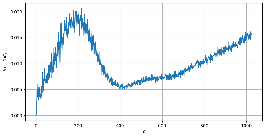
Spherical Harmonics transforms¶

healpy provides bindings to the C++ HEALPIX library for performing spherical harmonic transforms. hp.anafast computes the angular power spectrum of a map:

[21]:

LMAX = 1024
cl = hp.anafast(wmap_map_I_masked.filled(), lmax=LMAX)
ell = np.arange(len(cl))

therefore we can plot a normalized CMB spectrum and write it to disk:

[22]:

plt.figure(figsize=(10, 5))
plt.plot(ell, ell * (ell + 1) * cl)
plt.xlabel("$\ell$")
plt.ylabel("$\ell(\ell+1)C_{\ell}$")
plt.grid()
hp.write_cl("cl.fits", cl, overwrite=True)

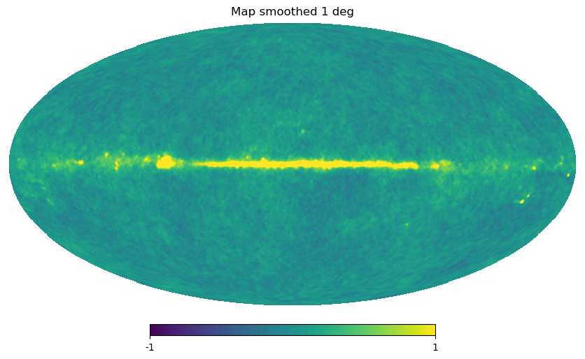
Gaussian beam map smoothing is provided by hp.smoothing:

[23]:

wmap_map_I_smoothed = hp.smoothing(wmap_map_I, fwhm=np.radians(1.))
hp.mollview(wmap_map_I_smoothed, min=-1, max=1, title="Map smoothed 1 deg")

For more information see the HEALPix primer

healpy tutorial¶

NSIDE and ordering¶

Reading and writing maps to file¶

Visualization¶

Spherical Harmonics transforms¶

healpy

Navigation

Related Topics